Macro Placement on the IBM/ICCAD04 Benchmarks
Adam Holmes · code on GitHub
A chip is millions of tiny logic cells plus a few hundred big fixed blocks — memory units and other
prebuilt components. Macro placement is deciding where those big blocks go, and it largely sets how
good the finished chip is. This is my solver for a benchmark challenge that grades each placement with a
single number — mostly wirelength, plus density and routing congestion; lower is better, no blocks may
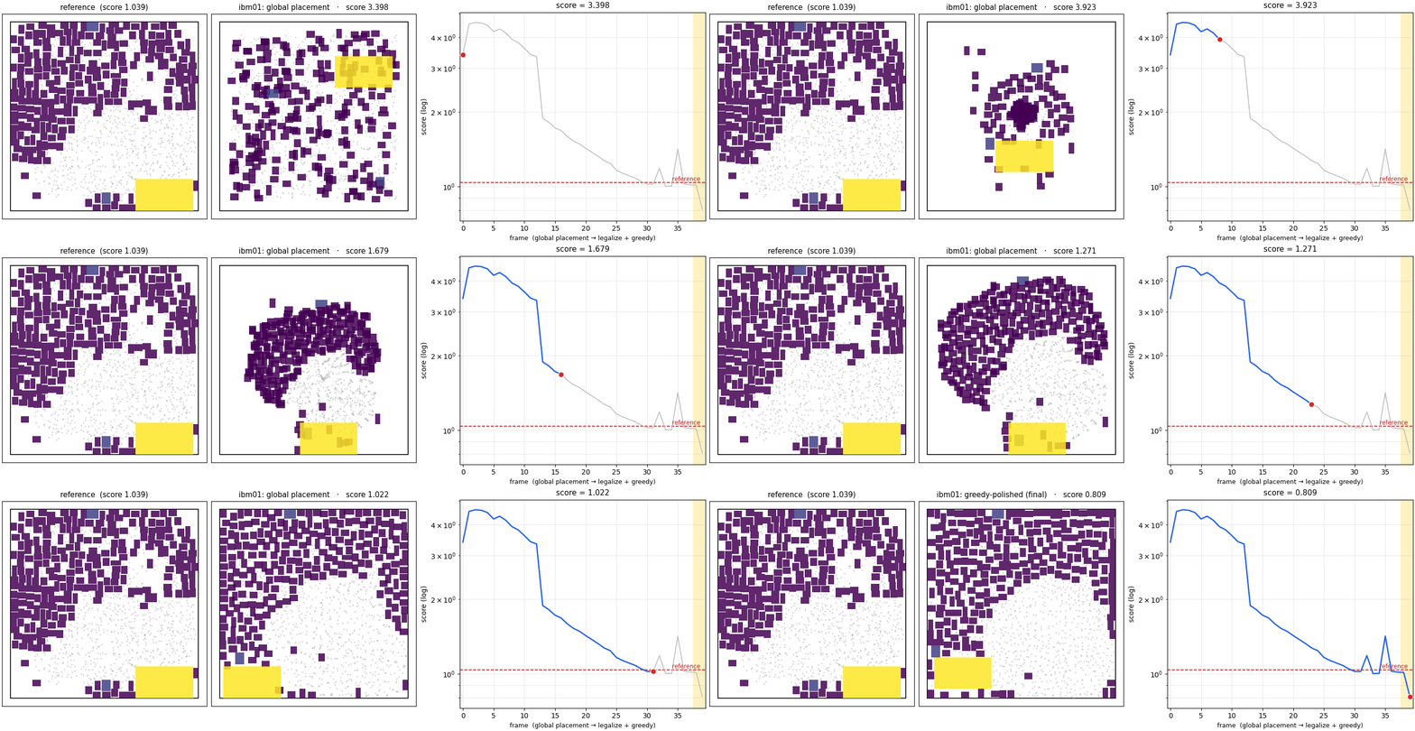
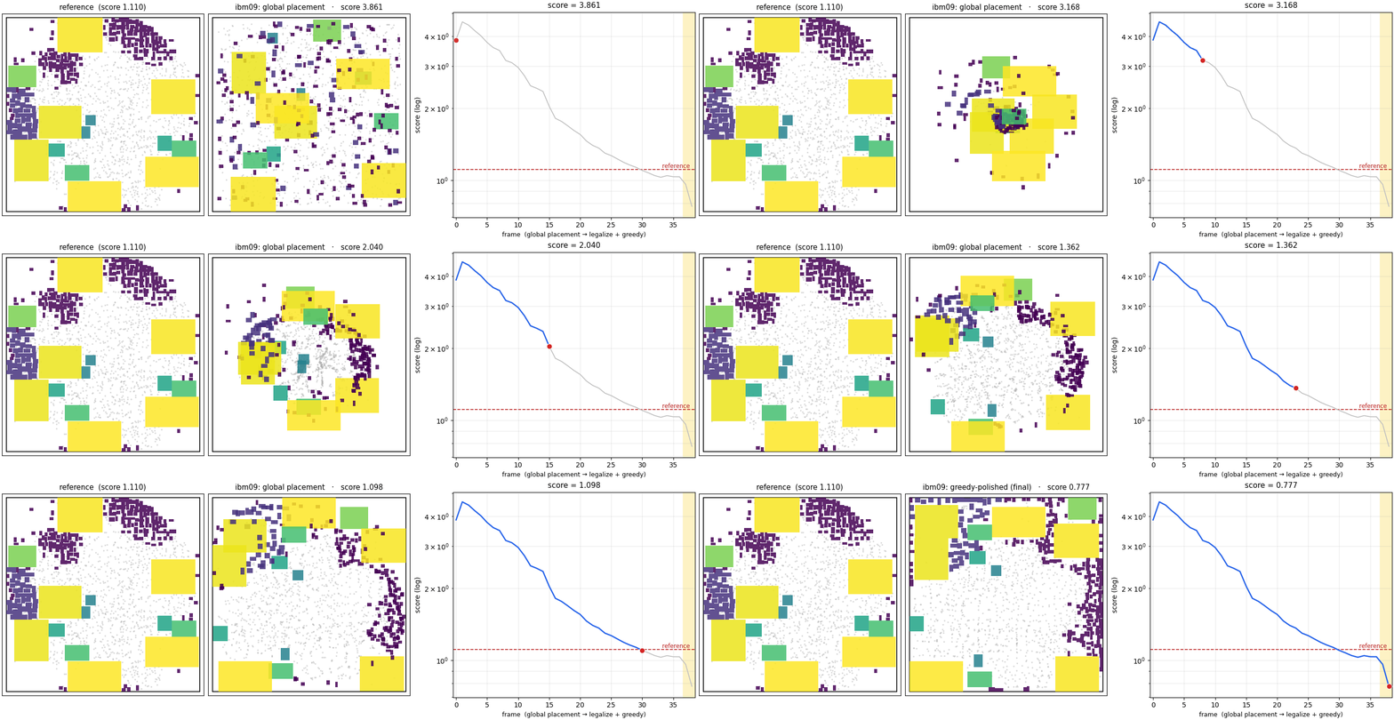
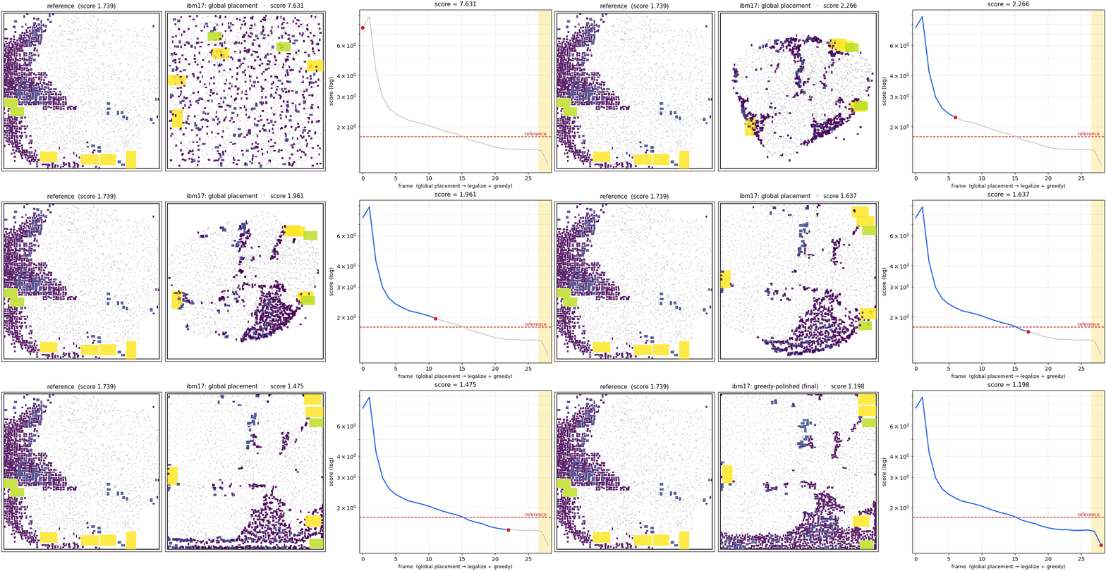
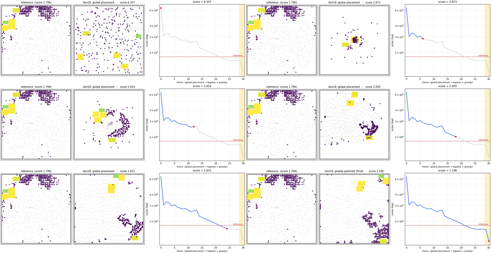
overlap. The animations replay real runs: the reference placement each benchmark comes with (left), my
placer working (middle), and the score per frame (right; dashed line = reference). Big blocks are
rectangles, cell clusters are dots. The small late bumps are schedule transients — the loss weights ramp up
sharply near the end and the score briefly rises while the layout reorganizes.
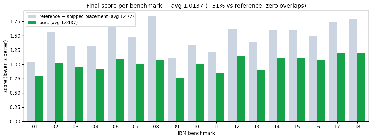
Result. From random starting placements, my pipeline averages 1.0137 over all 17
benchmarks — 31% below the provided reference (avg 1.477, a RePlAce-quality baseline; RePlAce itself
scores 1.458, simulated annealing 2.125), beating it on every design with zero overlaps. The design goal was
generality: the global placer optimizes any differentiable loss, so a new objective drops into the same
GPU engine unchanged.
Compute. A candidate takes ~3–6 min (GPU global stage ~80 s + CPU polish 1–5 min); the
1.0137 keeps the best of ~45 candidates per benchmark, generated within the challenge's 1-hour GPU budget with
the polish in parallel on CPU cores. A single candidate averages ~1.1. Scope: the score is dominated by
the movable standard-cell clusters — co-optimizing them drives ~98% of the gain, moving the big fixed blocks
only ~0.2%.
How it works
The score is 1.0·wirelength + 0.5·density + 0.5·congestion. Three stages, then a selection step:
- 1 · Differentiable global placement. Macro centers are free 2-D coordinates optimized by Adam
against a smooth stand-in for the score: per-net log-sum-exp wirelength and a grid-overflow density
penalty (the real terms aren't differentiable). The weights follow a schedule — loose early so connected
macros pull together, tightened late — which avoids the local optima a fully-on objective falls into.
- 2 · Legalization. Push overlapping blocks apart along their least-penetration axis, then a
cleanup pass that never worsens the score. Strict zero overlap on all 17.
- 3 · Greedy detailed placement. Single-macro moves accepted only if the true score
improves, ~1 ms/move on an exact-but-fast reimplementation of the metric (validated against the official
one). This closes the surrogate-to-true gap and does most of the absolute-quality work — 6.2% better
than running the same search from the reference.
- Multi-start. Random starts vary ~6%, so each design is placed from many seeds with a small pool
of configurations run side by side, keeping the per-design best — the gap between ~1.1 (one candidate)
and 1.0137. Different configurations win different designs (the tuned one below wins 11 of 17, the
tuning runners-up the rest). Past a few dozen candidates the gains flatten.
The tuned configuration
Two rounds of Bayesian optimization on 3 designs (ibm01/13/17 — easy/medium/hard; the other 14 held out),
scoring by average ratio to the reference. A first ~230-trial search on single-seed placements found the right
region; a warm-started ~115-trial second round then scored each candidate the way it's used — best of 3
seeds, after the greedy polish — with the winner confirmed at best-of-16:
| setting | value |
|---|
| wirelength sharpness | 2.44 (higher = closer to exact wirelength) |
| schedule back-loading | 3.99 (spread early, tighten late) |
| density weight (final / start) | 0.074 / ~3% of it · target fill 0.65, smoothing 0.17 |
| wirelength weight at start | 73% of full · learning rate 0.39 |
| overlap-tolerance window | deep-overlap penalty off for the first 6% of the run, full by 65% |
| same-size swaps | annealed swaps of equal-footprint macro pairs, active for the first third |
| diffusion term | searched, tuned to ≈0 (off) |
| gradient steps | 5000 in search → 15000 deployed (the knee of a later sweep; 30000 adds ≤1%) |
| not used | congestion term in the loss, electrostatic density, in-loss overlap resolution (appendix) |
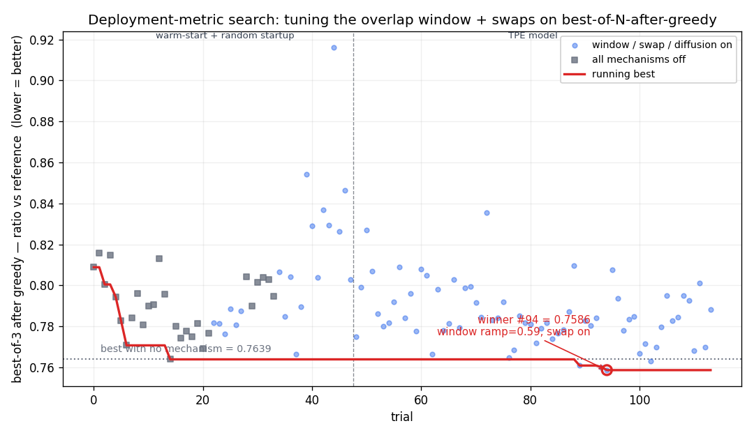
The second-round search. Squares = window/swaps/diffusion off, dots = on; the search plateaus
once differences between good configurations fall below the seed noise.
What I learned
- Multi-start beats a lucky seed. Single-seed scores carry ~2% noise — bigger than the gap between
good configurations — so single-seed rankings measure luck. Re-scoring the top five at best-of-16
reshuffled them and promoted a config that had ranked 5th. Every comparison here is paired on identical
seeds.
- Per-run tricks can't beat multi-start. The gradient stage mostly spreads macros and rarely
reorders them past each other, so I built four mechanisms to fix that (window, jumps, noise, swaps —
appendix). Each improves the typical run; none beats best-of-N. A paired variance test
shows why: they make runs converge (up to ~10× lower spread), but best-of-N wants the best of
many, and the random-start spread already contains one at least as good. The winning config earns its 11
designs because the swaps make it high-variance — a fatter tail to pick from. The random-start
variance isn't noise to remove; it's the search.
- It generalizes. The first-round config frozen and applied unchanged: 0.923 mean ratio on the 14
held-out designs vs 0.885 on the 3 tuning designs — a mild ~4-point overfit; 16 of 17 beat the reference
without any per-design selection.
- Congestion is the wall. At my best point it's 57% of the remaining cost and the term greedy
reduces least — it depends on discrete routing, not smoothly on positions. The ~7% gap to the
leaderboard leaders (~0.951) sits on the congestion-bound designs (ibm08/17/18). Single-macro greedy
plateaus there for a mechanical reason: relieving a hot region needs moving groups of cells
coherently, but any single move out of a crowded spot lengthens its own wires and is rejected. The
lever is coordinated multi-cell moves — not more tuning or congestion modeling.
Appendix — what didn't work
All paired experiments (identical seeds across arms) to cancel the ~2–6% seed noise.
- Congestion in the global loss. The metric is non-differentiable (discrete routing + a top-5%
mean), so I built two differentiable stand-ins. RUDY is gameable — the optimizer lowers it by spreading
nets while true congestion rises (correlation ≈ 0). My L-route model is faithful (correlation 0.94–0.99
with the true metric) — and still doesn't help, under any of four schedules. Greedy already optimizes
true congestion directly; a global term adds nothing it lacks while spoiling the low-wirelength layout
it starts from.
- Congestion-directed greedy. Sending crowded macros toward empty space — negative: the long jump
lengthens the moved macro's own wires and gets rejected, wasting the move.
- Interleaving the stages. Alternating gradient steps and greedy moves (incl. annealed acceptance,
matched compute) never beats global-then-greedy. The stages are genuinely separate: coarse arrangement,
then fine detail.
- Breaking the random-start ordering. Four mechanisms, each with its own Bayesian search on the
best-of-N-after-greedy metric: the overlap-tolerance window (typical run ~5% better,
best-of-N unchanged), teleporting high-wirelength macros to their net centroids (helps
wirelength-bound designs, hurts congestion-bound), annealed noise with mobility ∝ 1/√area (a wash at
crossing scale; larger scatters), and annealed same-size swaps (reaches orderings single moves can't —
still no best-of-N gain). All four reduce the run-to-run variance best-of-N feeds on; the
window+swap config survives only as the pool's high-variance member.
- Also: electrostatic (ePlace-style) density — matched the simpler overflow penalty; resolving
overlap inside the loss — over-spreads (a separate legalizer is better); simulated annealing and
SA/greedy hybrids — no gain at matched compute; moving the big fixed blocks and swapping same-size
clusters in greedy — the score barely responds (~0.2%); orientation flips — negligible.